10:00
8 Mapping
8.1 Working with spatial data in R
Throughout this tutorial you will be using ESRI Health Facilities in Kenya data It covers all the health facilities in Kenya, with the agency they are run by, their facility type, and their location. This data was last updated in 2022.
We want to visualise, and better understand how many health facilities there are at the sub-county and county level, and what the distribution of the different types of facility there are. To achieve this we will have to import spatial data, manipulate it, create summary statistics, and then plot it.
The data has been tidied up and saved as a Comma Separated Value file (.csv). We can use read_csv to open it in R.
8.1.1 Exercise
- Create a new object called
healthby usingread_csv(). - Use
glimpse()orhead()to view the structure ofhealth.
Solution
health <- readr::read_csv("data/Health_facilities_-4126638174547585951.csv")Rows: 4867 Columns: 17
── Column specification ────────────────────────────────────────────────────────
Delimiter: ","
chr (9): Facility Name, Province, District, Division, LOCATION, Sub Location...
dbl (8): FID, Facility Number, HMIS, Facility Type, Latitude, Longitude, x, y
ℹ Use `spec()` to retrieve the full column specification for this data.
ℹ Specify the column types or set `show_col_types = FALSE` to quiet this message.Solution
health# A tibble: 4,867 × 17
FID `Facility Number` `Facility Name` HMIS Province District Division
<dbl> <dbl> <chr> <dbl> <chr> <chr> <chr>
1 1 2 BARGONI HEALTH CENT… 3606 COAST LAMU HINDI
2 2 3 FAZA HEALTH CENTRE 626 COAST LAMU FAZA
3 3 4 HINDI MAGOGONI DISP 0 COAST LAMU HINDI
4 4 5 HINDI PRISON DISP 615 COAST LAMU HINDI
5 5 6 HONGWE CATHOLIC HEA… 616 COAST LAMU MPEKETO…
6 6 7 ICHUNDWA DISP 625 COAST LAMU KIZINGI…
7 7 8 KIUNGA HEALTH CENTRE 627 COAST LAMU KIUNGA
8 8 9 KIWAYU DISP 618 COAST LAMU KIZINGI…
9 9 10 KIZINGITINI DISP 617 COAST LAMU KIZINGI…
10 10 11 LAKE KENYATTA HEALT… 2451 COAST LAMU MPEKETO…
# ℹ 4,857 more rows
# ℹ 10 more variables: LOCATION <chr>, `Sub Location` <chr>, Spatial_Re <chr>,
# `Facility Type` <dbl>, Agency <chr>, Latitude <dbl>, Longitude <dbl>,
# GlobalID <chr>, x <dbl>, y <dbl>health is currently just a data frame - it has not got an explicit geometry column which links observations to their geographic location. It does however contain several columns which can be used to convert it into a spatial data format.
We could use the various names of locations to use as locations. But we would have to find a pre-existing map which had coordinates for each location. These locations could also be quite imprecise.
Fortunately we have also been provided with columns recording the Latitude, and Longitude of each incident. We can use those to convert health into an sf object. To achieve this we will use the st_as_sf() function which takes the following arguments:
new_object <- st_as_sf(x = input_data_frame, coords = c("x_coordinate_column", "y_coordinate_column"), crs = 27700)8.1.2 Exercise
10:00
- Create a new object called
health_sfby convertinghealthusing thest_as_sf()function. - Use
glimpse()orhead()to viewhealth_sfstructure.
Solution
health_sf <- sf::st_as_sf(health, coords = c("Longitude","Latitude"), crs = 4326)
head(health_sf)
Simple feature collection with 6 features and 15 fields
Geometry type: POINT
Dimension: XY
Bounding box: xmin: 40.65767 ymin: -2.341627 xmax: 41.12397 ymax: -2.057423
Geodetic CRS: WGS 84
# A tibble: 6 × 16
FID `Facility Number` `Facility Name` HMIS Province District Division
<dbl> <dbl> <chr> <dbl> <chr> <chr> <chr>
1 1 2 BARGONI HEALTH CENTRE 3606 COAST LAMU HINDI
2 2 3 FAZA HEALTH CENTRE 626 COAST LAMU FAZA
3 3 4 HINDI MAGOGONI DISP 0 COAST LAMU HINDI
4 4 5 HINDI PRISON DISP 615 COAST LAMU HINDI
5 5 6 HONGWE CATHOLIC HEAL… 616 COAST LAMU MPEKETO…
6 6 7 ICHUNDWA DISP 625 COAST LAMU KIZINGI…
# ℹ 9 more variables: LOCATION <chr>, `Sub Location` <chr>, Spatial_Re <chr>,
# `Facility Type` <dbl>, Agency <chr>, GlobalID <chr>, x <dbl>, y <dbl>,
# geometry <POINT [°]>st_as_sf() converted the Latitude and Longitude columns to simple feature geometries and created a new column called geometry which holds spatial information for each row. Now that health is a spatial object we can plot it using the ggplot2 package. For now we will use the geom_sf() function which creates a quick map, using ggplot2's default settings. geom_sf() only needs to be supplied with a simple feature object and is very useful for quickly inspecting your data. To quickly plot multiple layers on the same map use geom_sf() + geom_sf().
8.1.3 Exercise
03:00
- Plot
health_sfusing thegeom_sf()function.
Solution
ggplot2::ggplot(health_sf) +
ggplot2::geom_sf() 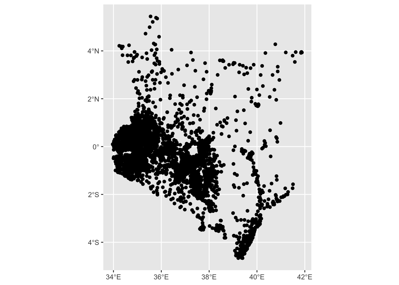
We can also create interactive maps using plotly or leaflet. For plotly we can write the map using ggplot2, before executing ggplotly().
8.1.4 Exercise
03:00
- Make an interactive map of
health_sfusing theggplotly()function.
Solution
ggplot_graph <- ggplot2::ggplot(health_sf) +
  ggplot2::geom_sf()

plotly::ggplotly(ggplot_graph)
8.2 Filtering by Administration Code
Our health facilities dataset covers all of Kenya. Let’s look at solely locations in Nairobi to narrow down our exploration more. To remove all points outside of Nairobi we will have to import a shapefile with the right county level and then use it to spatially filter our health_sf data.
So far we have created our own sf objects by adding a geometry column. The kenya data set is already a spatial one and as such we can use the st_read() function from the sf package to import it. st_read is extremely versatile and able to import most spatial data formats into R. The only argument that needs to be supplied to st_read is the fullpath to the file
8.2.1 Exercise
10:00
- You will need to download the Kenya shapefile. This is called
ken_adm_iebc_20191031_SHP.zipon the website. It will download a zip file, which you need to extract. You must extract the whole contents, as a shapefile is composed of multiple files. - Then, using
st_read, read inken_admbnda_adm2_iebc_20191031.shp, which is the shapefile containing the lowest level, subcounty boundaries. - Make a static map of the object you have just created using
geom_sf().
Solution
kenya_2017 <- sf::st_read("data/admn2/ken_admbnda_adm2_iebc_20191031.shp", quiet = TRUE)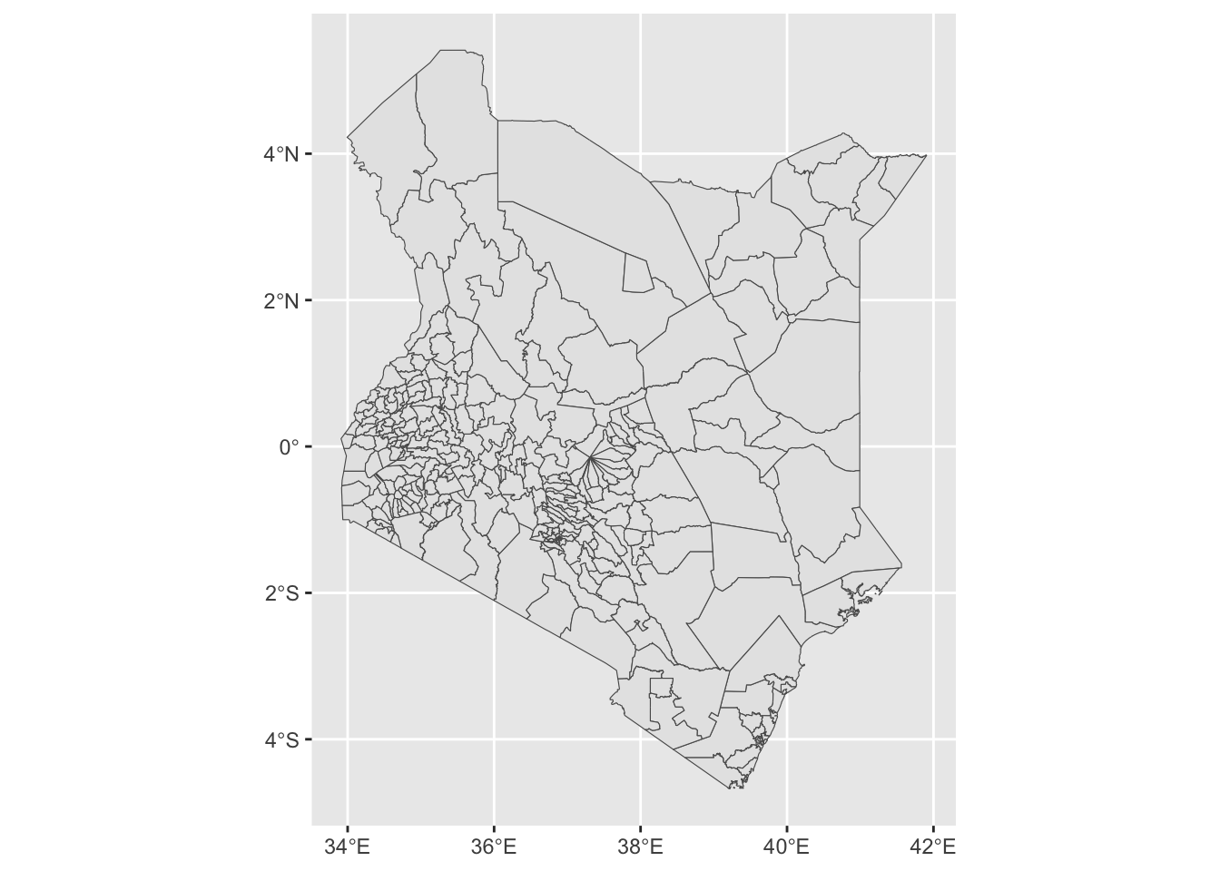
Sub-county level boundaries have loaded correctly but they currently cover all of Kenya. Because simple feature objects are data frames with a geometry column attached, any operations that we would perform on a normal data frame can also be performed on an object of class sf. We will use dplyr::filter and stringr::str_detect() to only keep sub-counties where their ADM1_PCODE code starts with KE047. KE047 denotes that an sub-county is part of Nairobi county.
8.2.2 Exercise
10:00
- Inspect kenya_2017 using
head()orglimpse(), and identify which column holds the county codes. - Create a new object called
nairobi_subcounty. Usedplyr::filteralongsidestringr::str_detect()to only keep observations which have a Administrative code starting with “KE047”. - Plot
nairobi_subcountyto see if the results look correct.
Solution
head(kenya_2017)Simple feature collection with 6 features and 14 fields
Geometry type: MULTIPOLYGON
Dimension: XY
Bounding box: xmin: 34.04426 ymin: -1.016204 xmax: 36.24609 ymax: 0.5589468
Geodetic CRS: WGS 84
Shape_Leng Shape_Area ADM2_EN ADM2_PCODE ADM2_REF ADM2ALT1EN ADM2ALT2EN
1 1.7469864 0.04082931 Ainabkoi KE027144 <NA> <NA> <NA>
2 0.9173066 0.01995665 Ainamoi KE035190 <NA> <NA> <NA>
3 1.4026374 0.03799999 Aldai KE029152 <NA> <NA> <NA>
4 1.0813543 0.04935731 Alego Usonga KE041234 <NA> <NA> <NA>
5 0.7439150 0.02136547 Awendo KE044254 <NA> <NA> <NA>
6 0.7970553 0.02423416 Bahati KE032174 <NA> <NA> <NA>
ADM1_EN ADM1_PCODE ADM0_EN ADM0_PCODE date validOn ValidTo
1 Uasin Gishu KE027 Kenya KE 2017-11-03 2019-10-31 -001-11-30
2 Kericho KE035 Kenya KE 2017-11-03 2019-10-31 -001-11-30
3 Nandi KE029 Kenya KE 2017-11-03 2019-10-31 -001-11-30
4 Siaya KE041 Kenya KE 2017-11-03 2019-10-31 -001-11-30
5 Migori KE044 Kenya KE 2017-11-03 2019-10-31 -001-11-30
6 Nakuru KE032 Kenya KE 2017-11-03 2019-10-31 -001-11-30
geometry
1 MULTIPOLYGON (((35.35933 0....
2 MULTIPOLYGON (((35.26262 -0...
3 MULTIPOLYGON (((34.93989 0....
4 MULTIPOLYGON (((34.20727 0....
5 MULTIPOLYGON (((34.54577 -0...
6 MULTIPOLYGON (((36.20478 -0...Solution
nairobi_subcounty <- dplyr::filter(kenya_2017, stringr::str_detect(ADM1_PCODE, "KE047"))
ggplot2::ggplot(nairobi_subcounty) +
ggplot2::geom_sf() 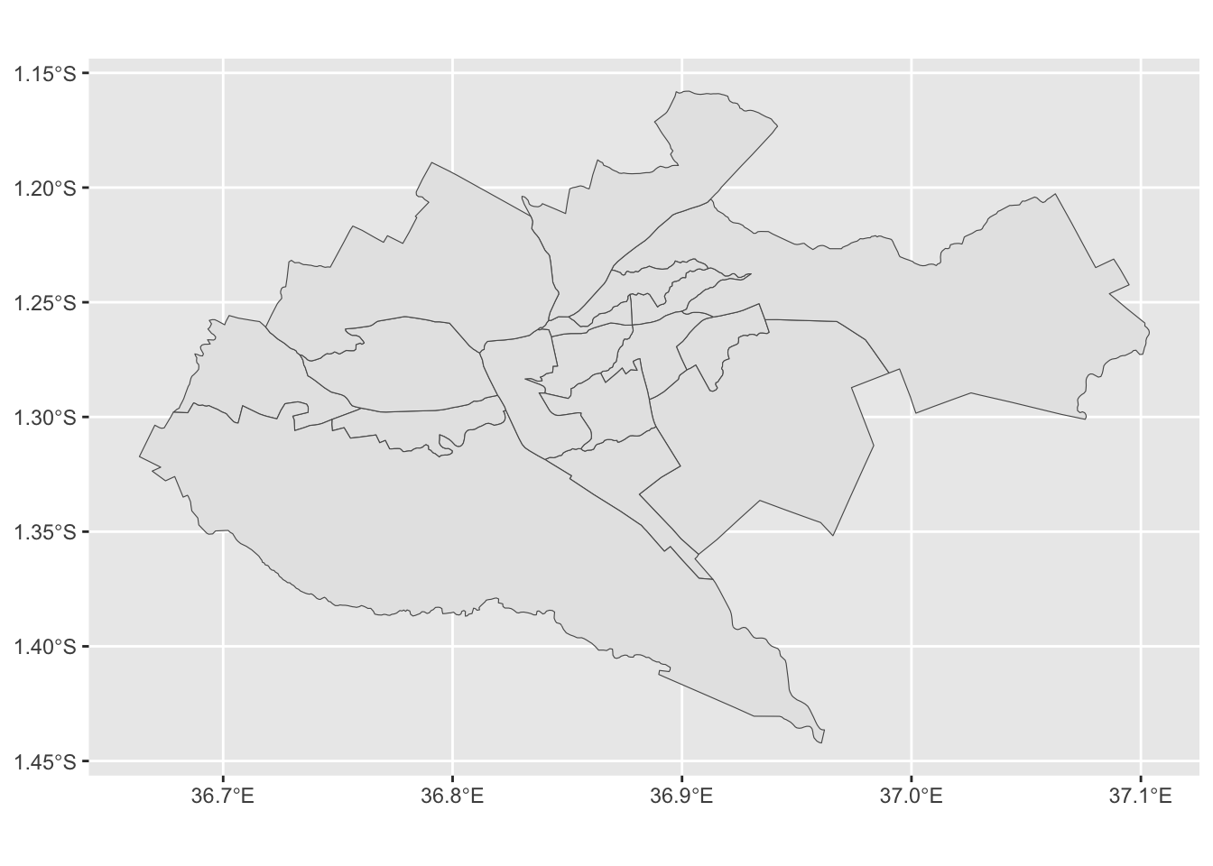
Finally, for the next step, we only need the outer boundary of Nairobi - all the internal subcounty boundaries have to be removed and only the outer edges kept. sf has a function exactly for this purpose called st_union(). It only takes one argument, which is the sf object we want to merge.
8.2.3 Exercise
10:00
- Create a new object called
nairobi_boundaryusing thest_unionfunction. - Plot it to check the results.
Solution
nairobi_boundary <- sf::st_union(nairobi_subcounty)
ggplot2::ggplot(nairobi_boundary) +
ggplot2::geom_sf() 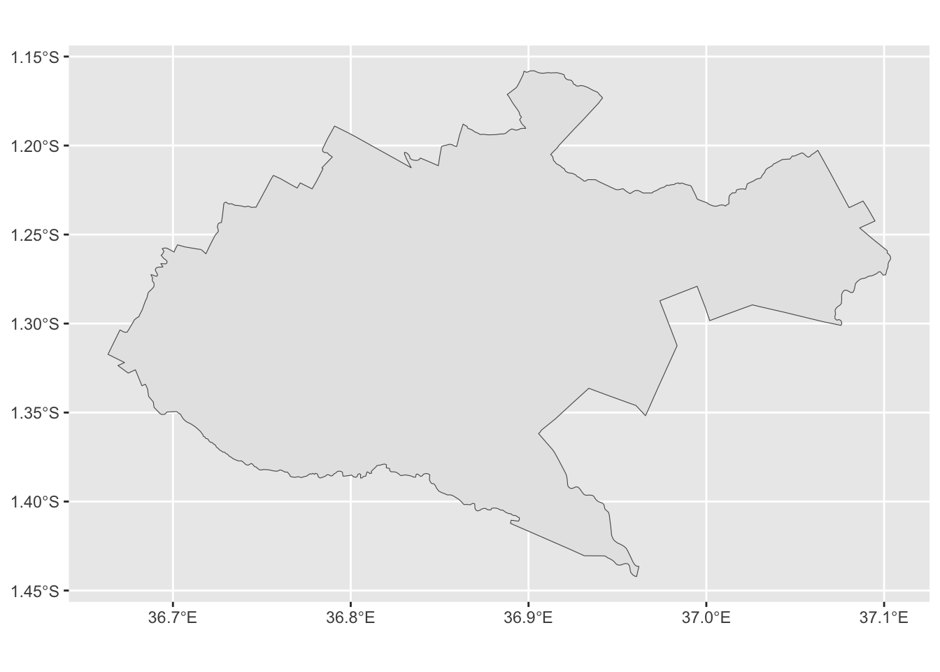
8.3 Spatial subsetting and CRS
In addition to subsetting by value, as we did with the Nairobi boundaries earlier, we can also subset observations by evaluating their spatial relationship with another data set. We can for example select all counties intersected by a river, or all households outside of city boundaries. There are a number of different spatial relationships which can be tested and used to subset observations.
sf has an inbuilt function called st_filter() which we can use to spatially subset observations. The function takes several arguments:
- x -
sfdata frame we want to subset -health_sf - y -
sfobject used to evaluate the spatial relationship -nairobi_boundary
Before running any spatial operations on two spatial objects it is always worth checking if their coordinate reference systems (CRS) match. sf will throw an error if that’s not the case. Try it for yourself below.
8.3.1 Exercise
10:00
- Use
st_filter()to spatially subsethealth_sfby testing its relationship withnairobi_boundary.
Solution
health_sf_nairobi <- st_filter(x = health_sf, y = nairobi_boundary)You should have got an error here saying x st_crs(x) == st_crs(y) is not TRUE. It means that objects x and y have different coordinate reference systems. Spatial operations require all objects to have the same CRS. We can see this for ourselves by running the st_crs() function, which returns the coordinate reference system of an object.
8.3.2 Exercise
03:00
- Run
st_crs()on both andhealth_sfandnairobi_boundaryand compare the results.
Solution
sf::st_crs(health_sf)[[1]][1] "EPSG:4326"Solution
sf::st_crs(nairobi_boundary)[[1]][1] "WGS 84"st_crs() provides detailed information about the CRS and projection of data, but all we need to check is its first element denoted by [[1]]. We can see that health_sf uses EPSG:4326, while nairobi_boundary is set to WGS 84. This problem can be solved by transforming nairobi_boundary’s CRS to match that of health_sf, simply by using the correct EPSG code. To do so we will use the st_transform() function which takes two arguments:
- x -
sfobject to be transformed - crs - EPSG code that we want to transform our data to - BNG is 4326
8.3.3 Exercise
10:00
- Run
st_transform()to transform and overwritenairobi_boundary. Remember to set the correct CRS. - Run
st_crs()onhealth_sfand newly transformednairobi_boundaryand compare the results.
Solution
nairobi_boundary <- sf::st_transform(nairobi_boundary, crs = 4326)

sf::st_crs(health_sf)[[1]]
[1] "EPSG:4326"Solution
sf::st_crs(nairobi_boundary)[[1]][1] "EPSG:4326"Now that the CRS are matching we should be able to spatially subset health_sf.
8.3.4 Exercise
10:00
- Use
st_filterto spatially subsethealth_sfby testing its relationship withnairobi_boundary. Overwritehealth_sfwith the subset data. - Plot it to check if the results are correct - all points should be within Nairobi
Solution
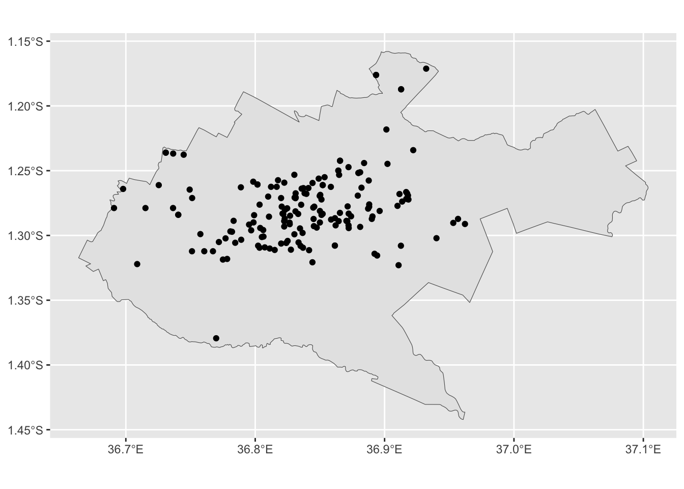
health_sf_filter <- sf::st_filter(x = health_sf, y = nairobi_boundary)
nairobi_map <- ggplot2::ggplot() +
  ggplot2::geom_sf(data = nairobi_boundary)  +
  ggplot2::geom_sf(data = health_sf_filter)