5  Tidy Data

5.1 What is tidy data anyway?

So far, your manipulation of data has focused on processes which make use of tidyverse functions, including filtering rows, selecting columns and creating new columns, as well as plotting data on charts. All of the functions you’ve seen have been easy to apply to the data you have.

Unfortunately, in real projects, this often won’t be the case because the data you’ll have often won’t be in tidy format, which is how most tidyverse functions expect to receive data.

Tidy data is a standardised structure of data designed make data cleaning and processing steps easy, and is straightforward even if it seems unusual at first.

You are likely to be most familiar with data laid out in a “messy” structure like the one below:

# A tibble: 30 × 8
   country                continent `1967` `1972` `1977` `1982` `1987` `1992`
   <fct>                  <fct>      <dbl>  <dbl>  <dbl>  <dbl>  <dbl>  <dbl>
 1 Albania                Europe      66.2   67.7   68.9   70.4   72     71.6
 2 Austria                Europe      70.1   70.6   72.2   73.2   74.9   76.0
 3 Belgium                Europe      70.9   71.4   72.8   73.9   75.4   76.5
 4 Bosnia and Herzegovina Europe      64.8   67.4   69.9   70.7   71.1   72.2
 5 Bulgaria               Europe      70.4   70.9   70.8   71.1   71.3   71.2
 6 Croatia                Europe      68.5   69.6   70.6   70.5   71.5   72.5
 7 Czech Republic         Europe      70.4   70.3   70.7   71.0   71.6   72.4
 8 Denmark                Europe      73.0   73.5   74.7   74.6   74.8   75.3
 9 Finland                Europe      69.8   70.9   72.5   74.6   74.8   75.7
10 France                 Europe      71.6   72.4   73.8   74.9   76.3   77.5
# ℹ 20 more rows

Here, the data has one row per country and then multiple columns, with one for each year. This may seem relatively logical and quite tidy, but the problems start when you realise that there are multiple other quite logical and tidy ways to lay this data out if there are few restrictions. For example, it could quite easily be shown with one country per column, and a year per row:

# A tibble: 12 × 143
    year Afghanistan Albania Algeria Angola Argentina Australia Austria Bahrain
   <int>       <dbl>   <dbl>   <dbl>  <dbl>     <dbl>     <dbl>   <dbl>   <dbl>
 1  1952        28.8    55.2    43.1   30.0      62.5      69.1    66.8    50.9
 2  1957        30.3    59.3    45.7   32.0      64.4      70.3    67.5    53.8
 3  1962        32.0    64.8    48.3   34        65.1      70.9    69.5    56.9
 4  1967        34.0    66.2    51.4   36.0      65.6      71.1    70.1    59.9
 5  1972        36.1    67.7    54.5   37.9      67.1      71.9    70.6    63.3
 6  1977        38.4    68.9    58.0   39.5      68.5      73.5    72.2    65.6
 7  1982        39.9    70.4    61.4   39.9      69.9      74.7    73.2    69.1
 8  1987        40.8    72      65.8   39.9      70.8      76.3    74.9    70.8
 9  1992        41.7    71.6    67.7   40.6      71.9      77.6    76.0    72.6
10  1997        41.8    73.0    69.2   41.0      73.3      78.8    77.5    73.9
11  2002        42.1    75.7    71.0   41.0      74.3      80.4    79.0    74.8
12  2007        43.8    76.4    72.3   42.7      75.3      81.2    79.8    75.6
# ℹ 134 more variables: Bangladesh <dbl>, Belgium <dbl>, Benin <dbl>,
#   Bolivia <dbl>, `Bosnia and Herzegovina` <dbl>, Botswana <dbl>,
#   Brazil <dbl>, Bulgaria <dbl>, `Burkina Faso` <dbl>, Burundi <dbl>,
#   Cambodia <dbl>, Cameroon <dbl>, Canada <dbl>,
#   `Central African Republic` <dbl>, Chad <dbl>, Chile <dbl>, China <dbl>,
#   Colombia <dbl>, Comoros <dbl>, `Congo, Dem. Rep.` <dbl>,
#   `Congo, Rep.` <dbl>, `Costa Rica` <dbl>, `Cote d'Ivoire` <dbl>, …

Having this kind of wide variety of potential structures means that when you receive data and try to use it, it’s almost impossible to have any kind of standardised approach to this non-standard data structuring. For example, if you want the most recent year of data from an annual dataset, would you need to select a column or filter some rows; it would depend entirely on the dataset!

In contrast, tidy data always has the same format:

• Every column is a variable.

• Every row is an observation.

• Every cell is a single value.

This is best explained in a tidy example:

# A tibble: 10 × 6
   country     continent  year lifeExp      pop gdpPercap
   <fct>       <fct>     <int>   <dbl>    <int>     <dbl>
 1 Afghanistan Asia       1952    28.8  8425333      779.
 2 Afghanistan Asia       1957    30.3  9240934      821.
 3 Afghanistan Asia       1962    32.0 10267083      853.
 4 Afghanistan Asia       1967    34.0 11537966      836.
 5 Afghanistan Asia       1972    36.1 13079460      740.
 6 Afghanistan Asia       1977    38.4 14880372      786.
 7 Afghanistan Asia       1982    39.9 12881816      978.
 8 Afghanistan Asia       1987    40.8 13867957      852.
 9 Afghanistan Asia       1992    41.7 16317921      649.
10 Afghanistan Asia       1997    41.8 22227415      635.

In this dataset, each column is a different variable; years, life expectancy, countries. These are best thought of as different categories that your data can fall into, not values of those categories. For example, year is a variable, but each possible year in that column is a value, and therefore shouldn’t be assigned its own column.

Every row is an observation; a unique combination of the variables included in the data. For example, there is only one observation (row) of data in Afghanistan for 1952, and then a separate one for the same country in 1957.

And importantly, there is only one value in each cell; this seems obvious but is suprisingly often not the case, especially when combined values such as age and sex (25M, 54F) or section and subsection (5b or 8c) are created.

5.2 Tidying messy data

Inevitably, you will often want to use data which is not in tidy format. Luckily the tidyverse package tidyr is designed to help with this, and contains a number of functions designed to tidy messy data. The functions you will want to use most frequently from this are the pivot verbs.

5.2.1 Pivot longer

The pivot_longer function does exactly what the name suggests, pivots data from a wide format (with many columns and few rows) to a long format (with many rows and few columns). This is very useful when you have data which has values as column names, and you want to gather these together into a single column of multiple values instead.

pay_gap <- read_csv('https://raw.githubusercontent.com/rfordatascience/tidytuesday/master/data/2022/2022-06-28/paygap.csv') |>
  select(employer_name, male_bonus_percent, female_bonus_percent,  date_submitted) 

This example uses the above dataset; a subsection UK company pay gap data, with male and female bonus percentages displayed in different columns. According to tidy data principles, this data would be easier to use if this data was stored in a single column with an additional variable indicating whether these were male or female bonuses.

Using pivot_longer we can specify the columns we’re talking about using the cols argument. This can be done in the same way as in the select function, either by specifying columns you wish to include or those you want to exclude (using the -).

There are several ways to use the pivot_longer function.

##Pivoting data; note that cols listed are the ones we want to include in the pivoting
pay_gap_long <- pay_gap |>
  pivot_longer(cols = c(male_bonus_percent, female_bonus_percent))

##Pivoting data; this returns the same result as the previous code, but the columns listed are excluded from the pivoting, so any not listed are pivoted
pay_gap_long <- pay_gap |>
  pivot_longer(cols = -c(employer_name,  date_submitted))

The other two arguments you may want to use are names_to and values_to, which allow you to specify the names of the columns you want to put the current column names (male_bonus_percent and female_bonus_percent) and values (the values in the two existing columns) into. If these are not specified, they will default to “name” and “value”, as in the examples above.

pay_gap_long <- pay_gap |>
  pivot_longer(cols = c(male_bonus_percent, female_bonus_percent),
                      names_to = "gender",
                      values_to = "percent")

5.2.2 Exercise

10:00

1. Using the inbuilt dataset billboard, pivot the week columns into a single long column. Call the dataset billboard_long

#Option 1: Excluding columns not being pivoted
billboard_long <- billboard |>
  pivot_longer(cols = -c(artist, track, date.entered),
               names_to = "week",
               values_to = "rank")

#Option 2: Specifying columns range explicitly
billboard_long <- billboard |>
  pivot_longer(cols = wk1:w76,
               names_to = "week",
               values_to = "rank")

#Option 3: Using starts_with()
billboard_long <- billboard |>
  pivot_longer(cols = starts_with("wk"), 
               names_to = "week",
               values_to = "rank")

5.3 Combining data tidying with data manipulation

The real power in tidy data comes with using it in combination with other dplyr verbs such as filtering, selecting and mutating. For example, in the full pay gap dataset, we can calculate whether there’s a difference in the hourly pay and bonuses by gender for different sizes of company:

pay_gap_summary <- read_csv('https://raw.githubusercontent.com/rfordatascience/tidytuesday/master/data/2022/2022-06-28/paygap.csv') |>
  #Select the columns we're interested in
  select(employer_name, diff_mean_hourly_percent, diff_mean_bonus_percent, employer_size) |>
  #Pivot to gather up all of the mean values into one column
  pivot_longer(cols = -c(employer_name, employer_size), names_to = "gender", values_to = "percent") |>
  #Group by employer size and variable type
  group_by(employer_size, gender) |>
  #Summarise by calculating means
  dplyr::summarise(percent = mean(percent, na.rm = TRUE)) |>
  #Remove companies which didn't specify a size
  filter(employer_size != "Not Provided")

5.4 Tidy data and plotting

The value of having a tidy dataset is also obvious when you come to plot your data in ggplot. Having a single variable in a column means that you’re able to assign that column to an aesthetic in ggplot, and therefore change the colour, shape, faceting, etc on the basis of that value! This opens the door to creating increasingly complex and informative (and pretty!) charts.

##Plot using the tidy data
ggplot(pay_gap_summary, aes(x = employer_size, 
                            y = percent, 
                            fill = gender))+ #Colours can be assigned to the different data types
  geom_col(position = "dodge") #makes bars sit next to eachother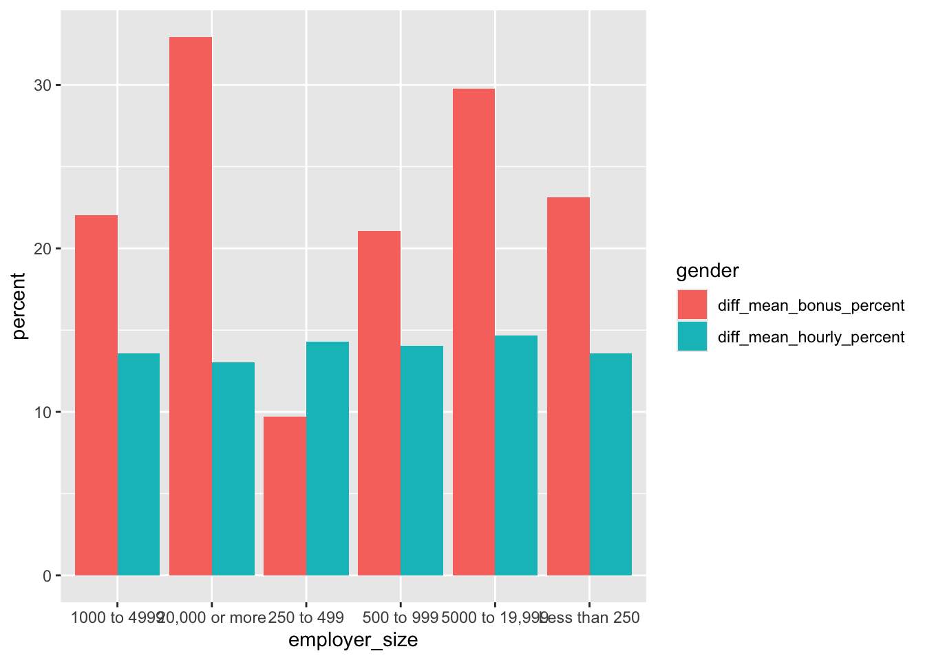

5.4.1 Exercise

15:00

1. Using the inbuilt dataset relig_income, pivot the income columns into a long dataset.
2. Assign this to an object called income_long
3. Using the dataset income_long you created, plot a bar chart in ggplot. Use religion as the x axis and the count of people as the y axis.
4. Assign the income groupings to the colour aesthetic.

#Tidy the data using pivot_longer()
income_long <- relig_income |>
  pivot_longer(cols = -religion,
               names_to = "income_group",
               values_to = "count")

#Plot your data 
income_chart <- 
  ggplot(income_long, aes(x = religion, y = count, fill = income_group)) +
  #stat = identity creates a stacked bar chart
  geom_bar(stat = "identity") +
  labs(x = "Religion", y = "Number of People", fill = "Income Group") +
  theme_minimal()

#print() allows you to view the chart in the 'Plots' tab
print(income_chart)

5.5 Multiple data frames

It’s rare that a data analysis involves only a single data frame. Typically you have many data frames, and you must join them together to answer the questions that you’re interested in.

In this lesson, you’ll learn about the most important types of joins, called Mutating joins. These joins add new variables to one data frame from matching observations in another.

5.6 Keys: Connecting your data frames

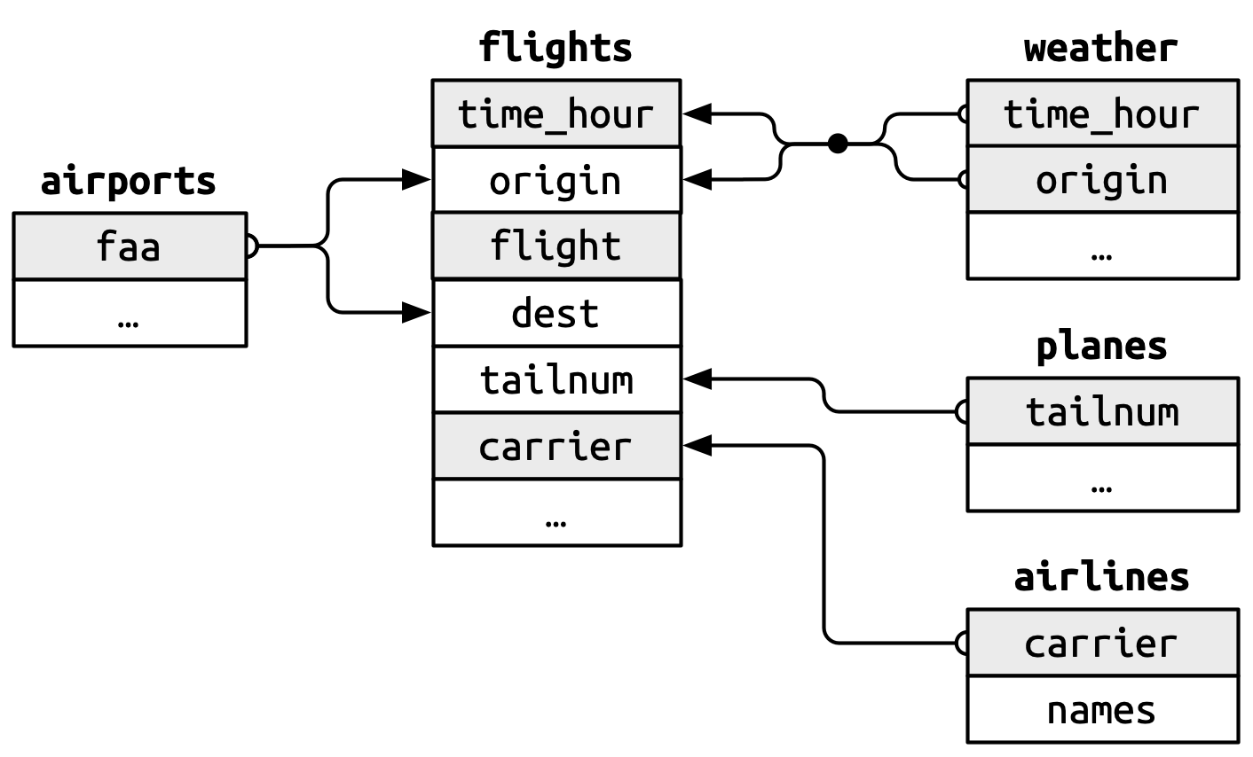
To understand joins, you need to first understand how two tables can be connected through a pair of keys. Every join involves a pair of keys:

A primary key is a variable or set of variables that uniquely identifies each observation. A foreign key is a variable (or set of variables) that corresponds to a primary key in another table.

When more than one variable is needed to form a key, it’s called a compound key. Let’s look at some examples from the nycflights13 package:

• airlines records two pieces of data about each airline: its carrier code and its full name. You can identify an airline with its two letter carrier code, making carrier the primary key.

  nycflights13::airlines

  # A tibble: 16 × 2
     carrier name                       
     <chr>   <chr>                      
   1 9E      Endeavor Air Inc.          
   2 AA      American Airlines Inc.     
   3 AS      Alaska Airlines Inc.       
   4 B6      JetBlue Airways            
   5 DL      Delta Air Lines Inc.       
   6 EV      ExpressJet Airlines Inc.   
   7 F9      Frontier Airlines Inc.     
   8 FL      AirTran Airways Corporation
   9 HA      Hawaiian Airlines Inc.     
  10 MQ      Envoy Air                  
  11 OO      SkyWest Airlines Inc.      
  12 UA      United Air Lines Inc.      
  13 US      US Airways Inc.            
  14 VX      Virgin America             
  15 WN      Southwest Airlines Co.     
  16 YV      Mesa Airlines Inc.         

• airports records data about each airport. You can identify each airport by its three letter airport code, making faa the primary key.

  airports

  # A tibble: 1,458 × 8
     faa   name                    lat    lon   alt    tz dst   tzone
     <chr> <chr>                 <dbl>  <dbl> <dbl> <dbl> <chr> <chr>
   1 04G   Lansdowne Airport      41.1  -80.6  1044    -5 A     Amer…
   2 06A   Moton Field Municipa…  32.5  -85.7   264    -6 A     Amer…
   3 06C   Schaumburg Regional    42.0  -88.1   801    -6 A     Amer…
   4 06N   Randall Airport        41.4  -74.4   523    -5 A     Amer…
   5 09J   Jekyll Island Airport  31.1  -81.4    11    -5 A     Amer…
   6 0A9   Elizabethton Municip…  36.4  -82.2  1593    -5 A     Amer…
   7 0G6   Williams County Airp…  41.5  -84.5   730    -5 A     Amer…
   8 0G7   Finger Lakes Regiona…  42.9  -76.8   492    -5 A     Amer…
   9 0P2   Shoestring Aviation …  39.8  -76.6  1000    -5 U     Amer…
  10 0S9   Jefferson County Intl  48.1 -123.    108    -8 A     Amer…
  # ℹ 1,448 more rows

• planes records data about each plane. You can identify a plane by its tail number, making tailnum the primary key.

  planes

  # A tibble: 3,322 × 9
     tailnum  year type        manufacturer model engines seats speed
     <chr>   <int> <chr>       <chr>        <chr>   <int> <int> <int>
   1 N10156   2004 Fixed wing… EMBRAER      EMB-…       2    55    NA
   2 N102UW   1998 Fixed wing… AIRBUS INDU… A320…       2   182    NA
   3 N103US   1999 Fixed wing… AIRBUS INDU… A320…       2   182    NA
   4 N104UW   1999 Fixed wing… AIRBUS INDU… A320…       2   182    NA
   5 N10575   2002 Fixed wing… EMBRAER      EMB-…       2    55    NA
   6 N105UW   1999 Fixed wing… AIRBUS INDU… A320…       2   182    NA
   7 N107US   1999 Fixed wing… AIRBUS INDU… A320…       2   182    NA
   8 N108UW   1999 Fixed wing… AIRBUS INDU… A320…       2   182    NA
   9 N109UW   1999 Fixed wing… AIRBUS INDU… A320…       2   182    NA
  10 N110UW   1999 Fixed wing… AIRBUS INDU… A320…       2   182    NA
  # ℹ 3,312 more rows
  # ℹ 1 more variable: engine <chr>

• weather records data about the weather at the origin airports. You can identify each observation by the combination of location and time, making origin and time_hour the compound primary key.

  weather

  # A tibble: 26,115 × 15
     origin  year month   day  hour  temp  dewp humid wind_dir
     <chr>  <int> <int> <int> <int> <dbl> <dbl> <dbl>    <dbl>
   1 EWR     2013     1     1     1  39.0  26.1  59.4      270
   2 EWR     2013     1     1     2  39.0  27.0  61.6      250
   3 EWR     2013     1     1     3  39.0  28.0  64.4      240
   4 EWR     2013     1     1     4  39.9  28.0  62.2      250
   5 EWR     2013     1     1     5  39.0  28.0  64.4      260
   6 EWR     2013     1     1     6  37.9  28.0  67.2      240
   7 EWR     2013     1     1     7  39.0  28.0  64.4      240
   8 EWR     2013     1     1     8  39.9  28.0  62.2      250
   9 EWR     2013     1     1     9  39.9  28.0  62.2      260
  10 EWR     2013     1     1    10  41    28.0  59.6      260
  # ℹ 26,105 more rows
  # ℹ 6 more variables: wind_speed <dbl>, wind_gust <dbl>,
  #   precip <dbl>, pressure <dbl>, visib <dbl>, time_hour <dttm>

The foreign keys in the flights dataset connect to the primary keys of these other tables:

flights$tailnumconnects to planes$tailnum flights$carrier connects to airlines$carrier flights$origin and flights$dest connect to airports$faa flights$origin and flights$time_hour together connect to weather$origin and weather$time_hour

These relationships are summarized visually in Figure 5.1.

Figure 5.1: Connections between all five data frames in the nycflights13 package. Variables making up a primary key are colored grey, and are connected to their corresponding foreign keys with arrows.

5.6.1 Checking primary keys

It’s good practice to verify that primary keys truly uniquely identify each observation. One way to do that is to count the primary keys and look for entries where the count is greater than one. One way to do that is to count() the primary keys and look for entries where n is greater than one. This reveals that planes and weather both look good:

planes |> 
  count(tailnum) |> 
  filter(n > 1)

# A tibble: 0 × 2
# ℹ 2 variables: tailnum <chr>, n <int>

weather |> 
  count(time_hour, origin) |> 
  filter(n > 1)

# A tibble: 0 × 3
# ℹ 3 variables: time_hour <dttm>, origin <chr>, n <int>

You should also check for missing values in your primary keys — if a value is missing then it can’t identify an observation!

planes |> 
  filter(is.na(tailnum))

# A tibble: 0 × 9
# ℹ 9 variables: tailnum <chr>, year <int>, type <chr>, manufacturer <chr>,
#   model <chr>, engines <int>, seats <int>, speed <int>, engine <chr>

weather |> 
  filter(is.na(time_hour) | is.na(origin))

# A tibble: 0 × 15
# ℹ 15 variables: origin <chr>, year <int>, month <int>, day <int>, hour <int>,
#   temp <dbl>, dewp <dbl>, humid <dbl>, wind_dir <dbl>, wind_speed <dbl>,
#   wind_gust <dbl>, precip <dbl>, pressure <dbl>, visib <dbl>,
#   time_hour <dttm>

5.6.2 Exercise

10:00

1. weather only contains information for the three origin airports in NYC. If it contained weather records for all airports in the USA, what additional connection would it make to flights?

# 1. weather$origin would join with flights%origin

5.7 Basic joins

Now that you understand how data frames are connected via keys, we can start using joins to better understand the flights dataset. dplyr provides six join functions:

• left_join(): keeps all observations in the first table
• inner_join(): keeps only observations that appear in both tables
• right_join(): keeps all observations in the second table
• full_join(): keeps all observations in either table
• semi_join(): filters the first table to include only observations that match the second table
• anti_join(): filters the first table to include only observations that don’t match the second table

In this course, you’ll learn how to use one mutating join, left_join(), and two filtering joins, semi_join() and anti_join().

5.7.1 Mutating joins

A mutating join allows you to combine variables from two data frames: it first matches observations by their keys, then copies across variables from one data frame to the other. Like mutate(), the join functions add variables to the right, so if your dataset has many variables, you won’t see the new ones. For these examples, we’ll make it easier to see what’s going on by creating a narrower dataset with just six variables.

flights2 <- flights |> 
  select(year, time_hour, origin, dest, tailnum, carrier)
flights2

# A tibble: 336,776 × 6
    year time_hour           origin dest  tailnum carrier
   <int> <dttm>              <chr>  <chr> <chr>   <chr>  
 1  2013 2013-01-01 05:00:00 EWR    IAH   N14228  UA     
 2  2013 2013-01-01 05:00:00 LGA    IAH   N24211  UA     
 3  2013 2013-01-01 05:00:00 JFK    MIA   N619AA  AA     
 4  2013 2013-01-01 05:00:00 JFK    BQN   N804JB  B6     
 5  2013 2013-01-01 06:00:00 LGA    ATL   N668DN  DL     
 6  2013 2013-01-01 05:00:00 EWR    ORD   N39463  UA     
 7  2013 2013-01-01 06:00:00 EWR    FLL   N516JB  B6     
 8  2013 2013-01-01 06:00:00 LGA    IAD   N829AS  EV     
 9  2013 2013-01-01 06:00:00 JFK    MCO   N593JB  B6     
10  2013 2013-01-01 06:00:00 LGA    ORD   N3ALAA  AA     
# ℹ 336,766 more rows

There are four types of mutating join, but there’s one that you’ll use almost all of the time: left_join(). It’s special because the output will always have the same rows as x, the data frame you’re joining to. The primary use of left_join() is to add in additional metadata. For example, we can use left_join() to add the full airline name to the flights2 data:

flights2 |>
  left_join(airlines)

Joining with `by = join_by(carrier)`

# A tibble: 336,776 × 7
    year time_hour           origin dest  tailnum carrier name                  
   <int> <dttm>              <chr>  <chr> <chr>   <chr>   <chr>                 
 1  2013 2013-01-01 05:00:00 EWR    IAH   N14228  UA      United Air Lines Inc. 
 2  2013 2013-01-01 05:00:00 LGA    IAH   N24211  UA      United Air Lines Inc. 
 3  2013 2013-01-01 05:00:00 JFK    MIA   N619AA  AA      American Airlines Inc.
 4  2013 2013-01-01 05:00:00 JFK    BQN   N804JB  B6      JetBlue Airways       
 5  2013 2013-01-01 06:00:00 LGA    ATL   N668DN  DL      Delta Air Lines Inc.  
 6  2013 2013-01-01 05:00:00 EWR    ORD   N39463  UA      United Air Lines Inc. 
 7  2013 2013-01-01 06:00:00 EWR    FLL   N516JB  B6      JetBlue Airways       
 8  2013 2013-01-01 06:00:00 LGA    IAD   N829AS  EV      ExpressJet Airlines I…
 9  2013 2013-01-01 06:00:00 JFK    MCO   N593JB  B6      JetBlue Airways       
10  2013 2013-01-01 06:00:00 LGA    ORD   N3ALAA  AA      American Airlines Inc.
# ℹ 336,766 more rows

Or we could find out the temperature and wind speed when each plane departed:

flights2 |> 
  left_join(weather |> select(origin, time_hour, temp, wind_speed))

Joining with `by = join_by(time_hour, origin)`

# A tibble: 336,776 × 8
    year time_hour           origin dest  tailnum carrier  temp wind_speed
   <int> <dttm>              <chr>  <chr> <chr>   <chr>   <dbl>      <dbl>
 1  2013 2013-01-01 05:00:00 EWR    IAH   N14228  UA       39.0       12.7
 2  2013 2013-01-01 05:00:00 LGA    IAH   N24211  UA       39.9       15.0
 3  2013 2013-01-01 05:00:00 JFK    MIA   N619AA  AA       39.0       15.0
 4  2013 2013-01-01 05:00:00 JFK    BQN   N804JB  B6       39.0       15.0
 5  2013 2013-01-01 06:00:00 LGA    ATL   N668DN  DL       39.9       16.1
 6  2013 2013-01-01 05:00:00 EWR    ORD   N39463  UA       39.0       12.7
 7  2013 2013-01-01 06:00:00 EWR    FLL   N516JB  B6       37.9       11.5
 8  2013 2013-01-01 06:00:00 LGA    IAD   N829AS  EV       39.9       16.1
 9  2013 2013-01-01 06:00:00 JFK    MCO   N593JB  B6       37.9       13.8
10  2013 2013-01-01 06:00:00 LGA    ORD   N3ALAA  AA       39.9       16.1
# ℹ 336,766 more rows

Or what size of plane was flying:

flights2 |> 
  left_join(planes |> select(tailnum, type, engines, seats))

Joining with `by = join_by(tailnum)`

# A tibble: 336,776 × 9
    year time_hour           origin dest  tailnum carrier type     engines seats
   <int> <dttm>              <chr>  <chr> <chr>   <chr>   <chr>      <int> <int>
 1  2013 2013-01-01 05:00:00 EWR    IAH   N14228  UA      Fixed w…       2   149
 2  2013 2013-01-01 05:00:00 LGA    IAH   N24211  UA      Fixed w…       2   149
 3  2013 2013-01-01 05:00:00 JFK    MIA   N619AA  AA      Fixed w…       2   178
 4  2013 2013-01-01 05:00:00 JFK    BQN   N804JB  B6      Fixed w…       2   200
 5  2013 2013-01-01 06:00:00 LGA    ATL   N668DN  DL      Fixed w…       2   178
 6  2013 2013-01-01 05:00:00 EWR    ORD   N39463  UA      Fixed w…       2   191
 7  2013 2013-01-01 06:00:00 EWR    FLL   N516JB  B6      Fixed w…       2   200
 8  2013 2013-01-01 06:00:00 LGA    IAD   N829AS  EV      Fixed w…       2    55
 9  2013 2013-01-01 06:00:00 JFK    MCO   N593JB  B6      Fixed w…       2   200
10  2013 2013-01-01 06:00:00 LGA    ORD   N3ALAA  AA      <NA>          NA    NA
# ℹ 336,766 more rows

When left_join() fails to find a match for a row in x, it fills in the new variables with missing values. For example, there’s no information about the plane with tail number N3ALAA so the type, engines, and seats will be missing:

flights2 |> 
  filter(tailnum == "N3ALAA") |> 
  left_join(planes |> select(tailnum, type, engines, seats))

Joining with `by = join_by(tailnum)`

# A tibble: 63 × 9
    year time_hour           origin dest  tailnum carrier type  engines seats
   <int> <dttm>              <chr>  <chr> <chr>   <chr>   <chr>   <int> <int>
 1  2013 2013-01-01 06:00:00 LGA    ORD   N3ALAA  AA      <NA>       NA    NA
 2  2013 2013-01-02 18:00:00 LGA    ORD   N3ALAA  AA      <NA>       NA    NA
 3  2013 2013-01-03 06:00:00 LGA    ORD   N3ALAA  AA      <NA>       NA    NA
 4  2013 2013-01-07 19:00:00 LGA    ORD   N3ALAA  AA      <NA>       NA    NA
 5  2013 2013-01-08 17:00:00 JFK    ORD   N3ALAA  AA      <NA>       NA    NA
 6  2013 2013-01-16 06:00:00 LGA    ORD   N3ALAA  AA      <NA>       NA    NA
 7  2013 2013-01-20 18:00:00 LGA    ORD   N3ALAA  AA      <NA>       NA    NA
 8  2013 2013-01-22 17:00:00 JFK    ORD   N3ALAA  AA      <NA>       NA    NA
 9  2013 2013-10-11 06:00:00 EWR    MIA   N3ALAA  AA      <NA>       NA    NA
10  2013 2013-10-14 08:00:00 JFK    BOS   N3ALAA  AA      <NA>       NA    NA
# ℹ 53 more rows

We’ll come back to this problem a few times in the rest of the chapter.

5.7.2 Specifying join keys

By default, left_join() will use all variables that appear in both data frames as the join key (a “natural join”). This is convenient but doesn’t always work. For example, if we try to join flights2 with the complete planes dataset:

flights2 |> 
  left_join(planes)

Joining with `by = join_by(year, tailnum)`

# A tibble: 336,776 × 13
    year time_hour           origin dest  tailnum carrier type  manufacturer
   <int> <dttm>              <chr>  <chr> <chr>   <chr>   <chr> <chr>       
 1  2013 2013-01-01 05:00:00 EWR    IAH   N14228  UA      <NA>  <NA>        
 2  2013 2013-01-01 05:00:00 LGA    IAH   N24211  UA      <NA>  <NA>        
 3  2013 2013-01-01 05:00:00 JFK    MIA   N619AA  AA      <NA>  <NA>        
 4  2013 2013-01-01 05:00:00 JFK    BQN   N804JB  B6      <NA>  <NA>        
 5  2013 2013-01-01 06:00:00 LGA    ATL   N668DN  DL      <NA>  <NA>        
 6  2013 2013-01-01 05:00:00 EWR    ORD   N39463  UA      <NA>  <NA>        
 7  2013 2013-01-01 06:00:00 EWR    FLL   N516JB  B6      <NA>  <NA>        
 8  2013 2013-01-01 06:00:00 LGA    IAD   N829AS  EV      <NA>  <NA>        
 9  2013 2013-01-01 06:00:00 JFK    MCO   N593JB  B6      <NA>  <NA>        
10  2013 2013-01-01 06:00:00 LGA    ORD   N3ALAA  AA      <NA>  <NA>        
# ℹ 336,766 more rows
# ℹ 5 more variables: model <chr>, engines <int>, seats <int>, speed <int>,
#   engine <chr>

We get many missing matches because our join is trying to use both tailnum and year as a compound key. But these year columns mean different things: in flights%year, it’s the year the flight occurred; in planes$year, it’s the year the plane was built.

flights2 |> 
  left_join(planes, join_by(tailnum))

# A tibble: 336,776 × 14
   year.x time_hour           origin dest  tailnum carrier year.y type          
    <int> <dttm>              <chr>  <chr> <chr>   <chr>    <int> <chr>         
 1   2013 2013-01-01 05:00:00 EWR    IAH   N14228  UA        1999 Fixed wing mu…
 2   2013 2013-01-01 05:00:00 LGA    IAH   N24211  UA        1998 Fixed wing mu…
 3   2013 2013-01-01 05:00:00 JFK    MIA   N619AA  AA        1990 Fixed wing mu…
 4   2013 2013-01-01 05:00:00 JFK    BQN   N804JB  B6        2012 Fixed wing mu…
 5   2013 2013-01-01 06:00:00 LGA    ATL   N668DN  DL        1991 Fixed wing mu…
 6   2013 2013-01-01 05:00:00 EWR    ORD   N39463  UA        2012 Fixed wing mu…
 7   2013 2013-01-01 06:00:00 EWR    FLL   N516JB  B6        2000 Fixed wing mu…
 8   2013 2013-01-01 06:00:00 LGA    IAD   N829AS  EV        1998 Fixed wing mu…
 9   2013 2013-01-01 06:00:00 JFK    MCO   N593JB  B6        2004 Fixed wing mu…
10   2013 2013-01-01 06:00:00 LGA    ORD   N3ALAA  AA          NA <NA>          
# ℹ 336,766 more rows
# ℹ 6 more variables: manufacturer <chr>, model <chr>, engines <int>,
#   seats <int>, speed <int>, engine <chr>

Note that the year variables are disambiguated in the output with a suffix (year.x and year.y).

join_by(tailnum) is short for join_by(tailnum == tailnum). The latter form is useful when the key variables have different names in each table:

flights2 |> 
  left_join(airports, join_by(dest == faa))

# A tibble: 336,776 × 13
    year time_hour           origin dest  tailnum carrier name         lat   lon
   <int> <dttm>              <chr>  <chr> <chr>   <chr>   <chr>      <dbl> <dbl>
 1  2013 2013-01-01 05:00:00 EWR    IAH   N14228  UA      George Bu…  30.0 -95.3
 2  2013 2013-01-01 05:00:00 LGA    IAH   N24211  UA      George Bu…  30.0 -95.3
 3  2013 2013-01-01 05:00:00 JFK    MIA   N619AA  AA      Miami Intl  25.8 -80.3
 4  2013 2013-01-01 05:00:00 JFK    BQN   N804JB  B6      <NA>        NA    NA  
 5  2013 2013-01-01 06:00:00 LGA    ATL   N668DN  DL      Hartsfiel…  33.6 -84.4
 6  2013 2013-01-01 05:00:00 EWR    ORD   N39463  UA      Chicago O…  42.0 -87.9
 7  2013 2013-01-01 06:00:00 EWR    FLL   N516JB  B6      Fort Laud…  26.1 -80.2
 8  2013 2013-01-01 06:00:00 LGA    IAD   N829AS  EV      Washingto…  38.9 -77.5
 9  2013 2013-01-01 06:00:00 JFK    MCO   N593JB  B6      Orlando I…  28.4 -81.3
10  2013 2013-01-01 06:00:00 LGA    ORD   N3ALAA  AA      Chicago O…  42.0 -87.9
# ℹ 336,766 more rows
# ℹ 4 more variables: alt <dbl>, tz <dbl>, dst <chr>, tzone <chr>

flights2 |> 
  left_join(airports, join_by(origin == faa))

# A tibble: 336,776 × 13
    year time_hour           origin dest  tailnum carrier name         lat   lon
   <int> <dttm>              <chr>  <chr> <chr>   <chr>   <chr>      <dbl> <dbl>
 1  2013 2013-01-01 05:00:00 EWR    IAH   N14228  UA      Newark Li…  40.7 -74.2
 2  2013 2013-01-01 05:00:00 LGA    IAH   N24211  UA      La Guardia  40.8 -73.9
 3  2013 2013-01-01 05:00:00 JFK    MIA   N619AA  AA      John F Ke…  40.6 -73.8
 4  2013 2013-01-01 05:00:00 JFK    BQN   N804JB  B6      John F Ke…  40.6 -73.8
 5  2013 2013-01-01 06:00:00 LGA    ATL   N668DN  DL      La Guardia  40.8 -73.9
 6  2013 2013-01-01 05:00:00 EWR    ORD   N39463  UA      Newark Li…  40.7 -74.2
 7  2013 2013-01-01 06:00:00 EWR    FLL   N516JB  B6      Newark Li…  40.7 -74.2
 8  2013 2013-01-01 06:00:00 LGA    IAD   N829AS  EV      La Guardia  40.8 -73.9
 9  2013 2013-01-01 06:00:00 JFK    MCO   N593JB  B6      John F Ke…  40.6 -73.8
10  2013 2013-01-01 06:00:00 LGA    ORD   N3ALAA  AA      La Guardia  40.8 -73.9
# ℹ 336,766 more rows
# ℹ 4 more variables: alt <dbl>, tz <dbl>, dst <chr>, tzone <chr>

inner_join(), right_join(), full_join() have the same interface as left_join(). The difference is which rows they keep: left join keeps all the rows in x, the right join keeps all rows in y, the full join keeps all rows in either x or y, and the inner join only keeps rows that occur in both x and y. We’ll come back to these in more detail later.

5.7.3 Exercise

20:00

1. Using arrange(), find the 48 hours (over the course of the whole year) that have the worst delays. Cross-reference it with the weather data. Can you see any patterns?

2. Imagine you’ve found the top 10 most popular destinations using this code:

   top_dest <- flights2 |>
     count(dest, sort = TRUE) |>
     head(10)

   How can you find all flights to those destinations?

3. Does every departing flight have corresponding weather data for that hour?

5.8 How do joins work?

Now that you’ve used joins a few times it’s time to learn more about how they work, focusing on how each row in x matches rows in y. We’ll begin by introducing a visual representation of joins, using the simple tibbles defined below and shown in Figure 5.2. In these examples we’ll use a single key called key and a single value column (val_x and val_y), but the ideas all generalize to multiple keys and multiple values.

x <- tribble(
  ~key, ~val_x,
     1, "x1",
     2, "x2",
     3, "x3"
)
y <- tribble(
  ~key, ~val_y,
     1, "y1",
     2, "y2",
     4, "y3"
)

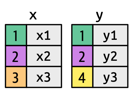
Figure 5.2: Graphical representation of two simple tables. The colored key columns map background color to key value. The grey columns represent the “value” columns that are carried along for the ride.

Figure 5.3 introduces the foundation for our visual representation. It shows all potential matches between x and y as the intersection between lines drawn from each row of x and each row of y. The rows and columns in the output are primarily determined by x, so the x table is horizontal and lines up with the output.

Figure 5.3: To understand how joins work, it’s useful to think of every possible match. Here we show that with a grid of connecting lines.

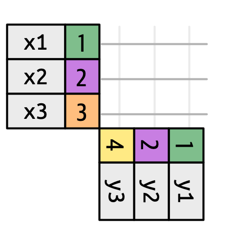
To describe a specific type of join, we indicate matches with dots. The matches determine the rows in the output, a new data frame that contains the key, the x values, and the y values. For example, Figure 5.4 shows an inner join, where rows are retained if and only if the keys are equal.

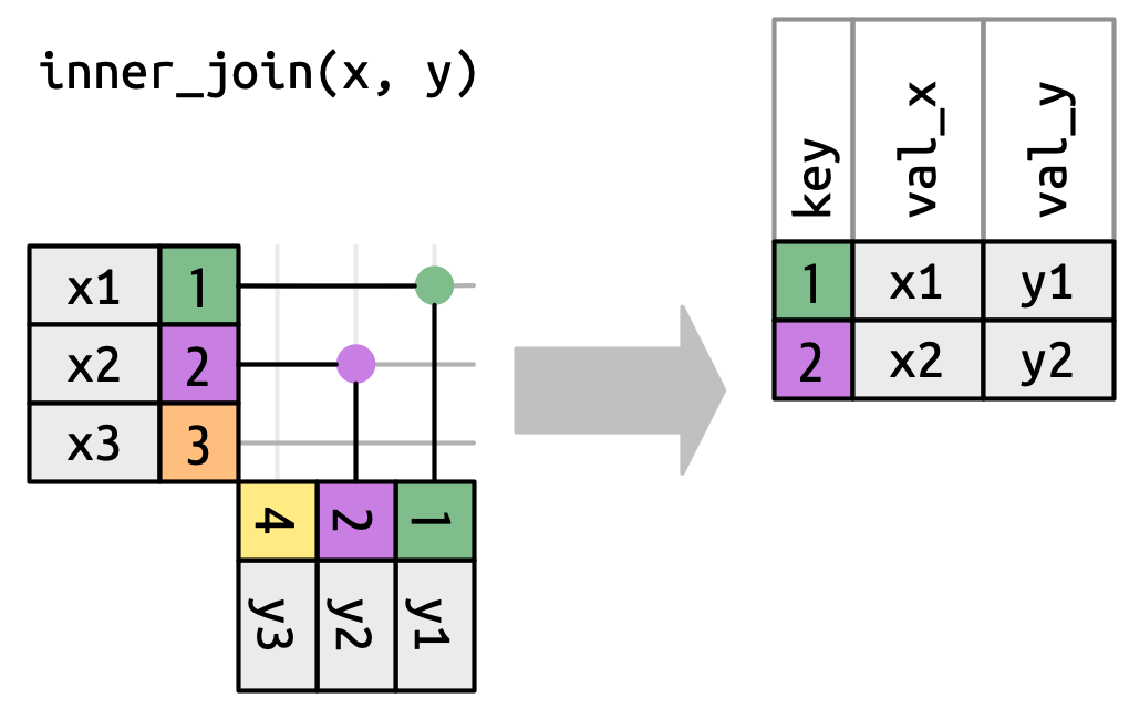
Figure 5.4: An inner join matches each row in x to the row in y that has the same value of key. Each match becomes a row in the output.

We can apply the same principles to explain the outer joins, which keep observations that appear in at least one of the data frames. These joins work by adding an additional “virtual” observation to each data frame. This observation has a key that matches if no other key matches, and values filled with NA. There are three types of outer joins:

• A left join keeps all observations in x, Figure 5.5. Every row of x is preserved in the output because it can fall back to matching a row of NAs in y.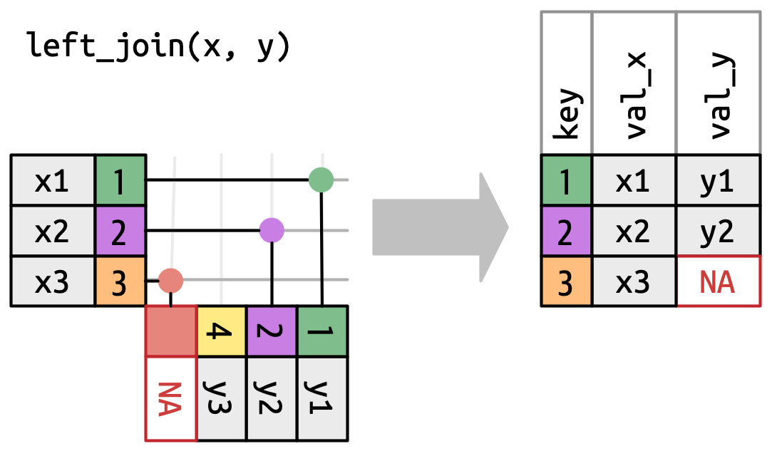

  

  Figure 5.5: A visual representation of the left join where every row in x appears in the output.

• A right join keeps all observations in y, Figure 5.6. Every row of y is preserved in the output because it can fall back to matching a row of NAs in x. The output still matches x as much as possible; any extra rows from y are added to the end.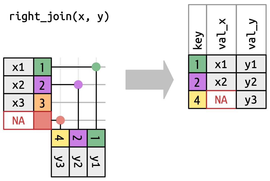

  

  Figure 5.6: A visual representation of the right join where every row of y appears in the output.

• A full join keeps all observations that appear in x or y, Figure 5.7. Every row of x and y is included in the output because both x and y have a fall back row of NAs. Again, the output starts with all rows from x, followed by the remaining unmatched y rows.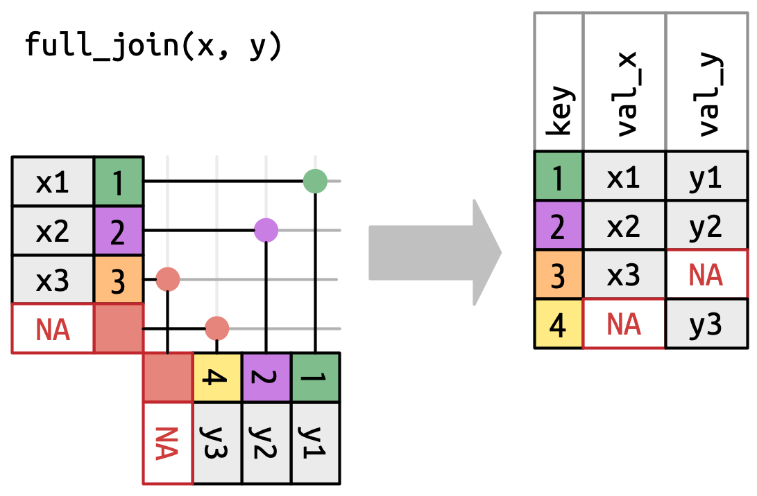

  

  Figure 5.7: A visual representation of the full join where every row in x and y appears in the output.

Another way to show how the types of outer join differ is with a Venn diagram, as in Figure 5.8. However, this is not a great representation because while it might jog your memory about which rows are preserved, it fails to illustrate what’s happening with the columns.

Figure 5.8: Venn diagrams showing the difference between inner, left, right, and full joins.

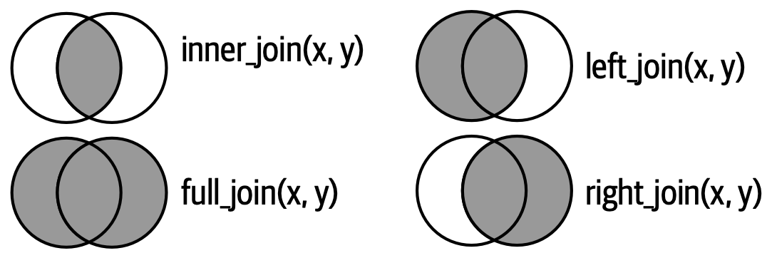
The joins shown here are the so-called equi joins, where rows match if the keys are equal. Equi joins are the most common type of join, so we’ll typically omit the equi prefix, and just say “inner join” rather than “equi inner join”.

5.8.1 Row matching

So far we’ve explored what happens if a row in x matches zero or one row in y. What happens if it matches more than one row? To understand what’s going on let’s first narrow our focus to the inner_join() and then draw a picture, Figure 5.9.

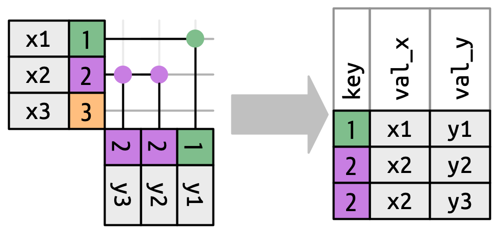
Figure 5.9: The three ways a row in x can match. x1 matches one row in y, x2 matches two rows in y, x3 matches zero rows in y. Note that while there are three rows in x and three rows in the output, there isn’t a direct correspondence between the rows.

There are three possible outcomes for a row in x:

• If it doesn’t match anything, it’s dropped.
• If it matches 1 row in y, it’s preserved.
• If it matches more than 1 row in y, it’s duplicated once for each match.

In principle, this means that there’s no guaranteed correspondence between the rows in the output and the rows in x, but in practice, this rarely causes problems. There is, however, one particularly dangerous case which can cause a combinatorial explosion of rows. Imagine joining the following two tables:

df1 <- tibble(key = c(1, 2, 2), val_x = c("x1", "x2", "x3"))
df2 <- tibble(key = c(1, 2, 2), val_y = c("y1", "y2", "y3"))

While the first row in df1 only matches one row in df2, the second and third rows both match two rows. This is sometimes called a many-to-many join, and will cause dplyr to emit a warning:

df1 |> 
  inner_join(df2, join_by(key))

Warning in inner_join(df1, df2, join_by(key)): Detected an unexpected many-to-many relationship between `x` and `y`.
ℹ Row 2 of `x` matches multiple rows in `y`.
ℹ Row 2 of `y` matches multiple rows in `x`.
ℹ If a many-to-many relationship is expected, set `relationship =
  "many-to-many"` to silence this warning.

# A tibble: 5 × 3
    key val_x val_y
  <dbl> <chr> <chr>
1     1 x1    y1   
2     2 x2    y2   
3     2 x2    y3   
4     2 x3    y2   
5     2 x3    y3   

If you are doing this deliberately, you can set relationship = "many-to-many", as the warning suggests.